Four-Dimensional Stock Market Structures and Cycles
Description of Lessons 1 – 10
Part One – Structures – (Lessons 1 – 5)
Lesson I – Provides a unique way to look at financial markets by defining Cowan’s ‘Price-Time Vector’. Mr. Cowan discovered this tool in the early 1980’s. It is used to reveal the four-dimensional structures hidden in traditional price-time charts.

Numerous examples and exercises are provided of this new method of viewing price-time charts. This lesson shows how to make predictions similar to W. D. Gann when he stated: “Union Pacific will not touch 169 before a big break.” He made this statement when Union Pacific was trading at 168 1/8. It never touched 169.
YouTube video: Pythagorean Theorem to Forecast…
Lesson II – Uses the tools developed in Lesson I to show the elliptical formations in price-time that contain the action. This provides the analyst with a very valuable technique for determining turning points in both price and time.
YouTube video: Ellipse in the New York Composite.
YouTube video: Ellipse in the Russell 2000.
Lesson III – Shows step by step how growth patterns unfold in financial markets.
The analyst is shown how “Dynamic Symmetry,” as practiced by the ancient Greeks, is used to identify terminal points of the growth process. Although contemporary market analysts try to force price-time data into a Fibonacci growth spiral, this number series is NOT the one upon which stock market growth spirals are based. The true growth spiral is identified.
YouTube video: Growth Spirals and Gravity Wells
Lesson IV– Titled, “Price-Time Ratios More Important Than Fibonacci,” this lesson provides detailed examples of the four most important ratios in financial market timing. All four are more important than the famed Fibonacci ratio. Contemporary analysts who are using the Fibonacci ratio to project retracement values typically apply this ratio to every downturn in the market.

Lesson V – Uses the information from the first four lessons to clearly describe the geometric structures in the stock market, since the year 1790. This is first shown in two dimensions. Then progressively evolved to a three-dimensional and finally a four-dimensional geometric structure.
Without knowledge of the geometric structure being formed, accurate cycle projections are difficult because a cycle’s periodicity and phase changes when the face of the structure completes.
Part Two – Cycles – (Lessons 6 – 10)
Lesson VI – Explains the “Law of Vibration.” W. D. Gann stated, “I have proven to my entire satisfaction as well as demonstrated to others, that the Law of Vibration explains every possible phase and condition of the market.” This is a simple scientific principle which few people have realized also applies to financial markets. However, financial markets are not exempt from any natural law.
Lesson VII – Titled, “Cycles,” this lesson describes what a cycle really is, how varying energy levels define the duration and magnitude of these cycles, and solves the two age-old problems of: (1) varying periodicity of cycle tops and bottoms; (2) why cycles “disappear” then reappear with phase shifts. This is NOT caused by the phenomenon of “beats,” i.e., cycles interfering destructively.
 The subject of financial market cycles is little understood by most analysts.
The traditional methods of Fourier Transforms and percent deviations from moving averages originated with scientists and engineers. While these techniques are effective in isolating individual cyclic components of such things as radio waves or compound sound waves, they are little help when the complex topic of repetitive human behavior is studied. The cyclic component of mass human psychology becomes evident as men repeat the same mistakes committed by their parents and grandparents. When measured in mass, man not only seems incapable of learning from the mistakes of history, but also inclined to repeat the errors committed as recently as the previous generation.

Lesson VIII – Applies the scientific phenomenon known as “sympathetic resonance” to demonstrate the cause of every stock market cycle greater than six weeks. Legendary traders such as W. D. Gann and George Bayer used the motions of the planets as a timing tool. However, until now, no one has discovered the methods these traders were actually using. This lesson identifies the synchronicity that exists between planetary cycles and stock market cycles, with complete historical analysis for each cycle. The analysis of the longer cycles extends back to 1790 for the stock market.
YouTube video: Saturn-Uranus Stock Market Cycle
Lesson IX -Uses all information previously presented to create models projecting price-time action. One example of the results obtained is the five-year stock market model shown here.
The top line is the model that was created in 1984 to project the stock market for the next several years. The bottom line is what actually happened.
EVERY TURNING POINT WAS PREDICTED BY THIS MODEL, i.e., the bottom in August, 1982; the top in January, 1984; the bottom in July, 1984; the bottom in September, 1985; the sideways churning market during March-September, 1986; the major top in August, 1987; and the “crash of October 1987”.
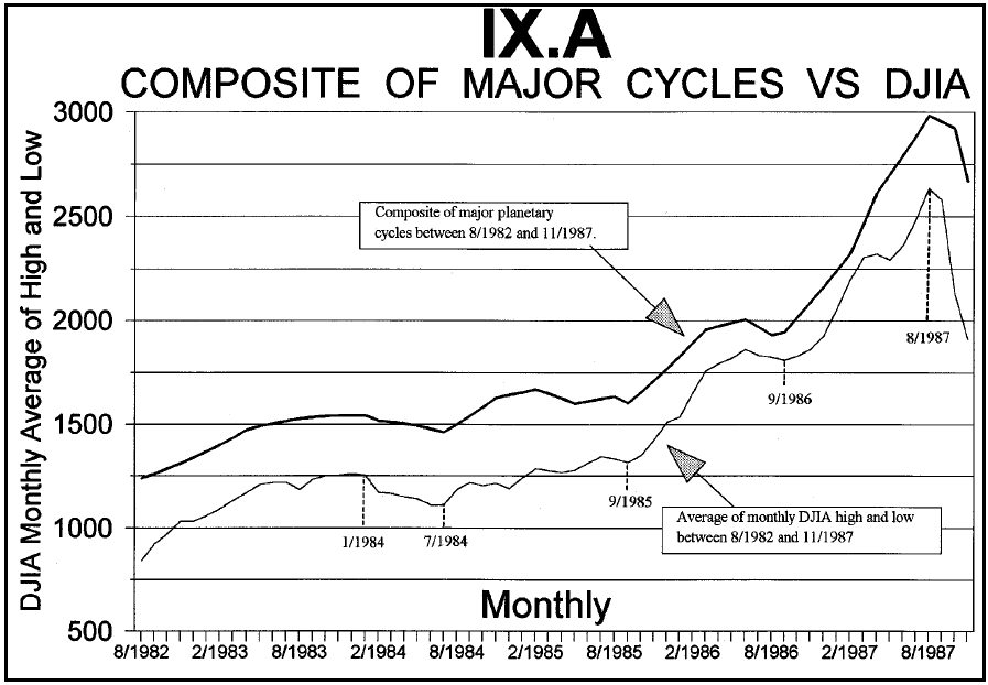
Lesson IX walks you through the process step-by-step that was used to create this model.
The same tools and techniques apply to price-time swings smaller than those shown in this figure.
Lesson X – Titled “Dimensional Aspects of Time,” this lesson provides the theoretical basis for the four-dimensional effects seen in financial markets. Traditional price-time charts misrepresent time by treating it as a single linear dimension along the bottom of the chart. Time is neither one-dimensional nor linear.